Robbins–Monro Root-Finding Structure

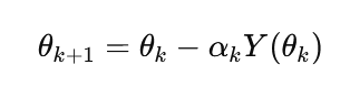
The Robbins–Monro procedure (1951) defines a stochastic approximation method for solving equations of the form:

where only noisy observations of Y(θ) are available. The iterative update takes the form:

with step sizes αk satisfying:

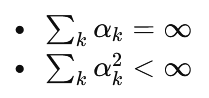
This ensures convergence under mild regularity conditions. The structure can be interpreted as a noisy root-finding scheme where each iteration moves the estimate toward a zero of the expected signal.

Use in Optimization

Optimization problems can be reformulated as root-finding tasks by targeting stationary points:

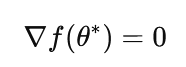
Replacing Y(θ) with a stochastic gradient estimator yields:

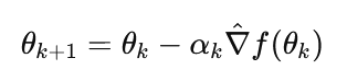
This connects Robbins–Monro directly to stochastic gradient descent (SGD). The method is particularly suited for settings where gradients are noisy, expensive, or only indirectly observable.

SPSA as a Variant

Simultaneous Perturbation Stochastic Approximation (SPSA), introduced by Spall, modifies the Robbins–Monro framework by replacing explicit gradient estimates with randomized finite differences. At each iteration:

1) A random perturbation vector Δk is sampled.

2) A gradient estimate is formed using:

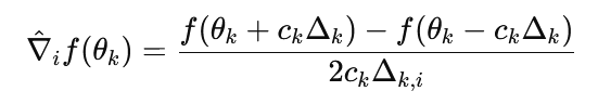
This requires only two function evaluations regardless of dimension, making SPSA efficient in high-dimensional settings. The update then follows the Robbins–Monro form.

Polyak–Ruppert Averaging

Following experimental results indicate that simple Polyak–Ruppert averaging outperforms both constant learning rate Robbins–Monro updates
and a carefully tuned SPSA implementations:

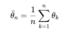
Polyak–Ruppert averaging computes the final estimate as the average of iterates:

In practice, suffix averaging is often used:

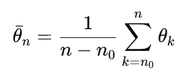
where n0 defines a so called "burn-in" or "warm-up" period.

In this particular example a cosine with noise is being optimized:

f[x_] := Cos[x] + RandomVariate[NormalDistribution[0, 0.5]]

Results: 

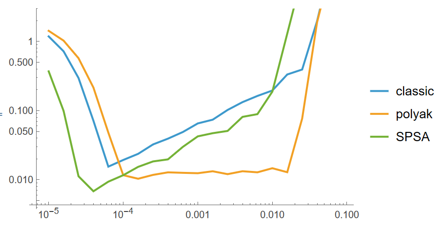
Figure 1: y-axis: Distance to the optimimum after 10^5 iterations averaged 100 times, x-axis: learning rate of the algorithm. 3 algorithms are compared: blue - default Robbins-Monroe update with constant learning rate, orange - Polyak-Ruppert suffix averaging, green - SPSA algorithm with paremeters tuned as recommended by Spall

Polyak-Ruppert style suffix averaging yields almost fully dominant results as compared to other algorithms. Good results can be achieved even with a constant learning rate as well as a wider learning rate convergence region.
There is no reason not to use it.